Compound Interest in a Bank
Assume the bank gives you interest of 100% per year, i.e., interest rate r = 1 over one year. The amount A in the bank at end of y years will be = 1, 2, 4, 8, 16, etc.
However, a deal is offered by the bank to increase your savings without increasing the total interest rate (r = 1). The bank would give you interest twice a year, but each time at half the annual interest rate. That is, every half year, the interest paid would be 0.5 of what you have in the bank at that time. If you invest with $1 to start, at half-year, your account will be $1.5; and at year end, your account will be $1.5 • 1.5 = $2.25. So, the account sequence is, for doubling and quadrupling the frequency of interest payments:
payment 1,2: A = 1.5, 2.25
payment 1,2,3,4: A = 1.25, 1.56, 1.95, 2.44
If the bank offers deals with more rapid growth, the resulting amounts can be calculated by the formula: 
p = 1,2: A = 1.5, 2.25
p = 1,2,4: A = 1.25, 1.56, 2.44
p = 1,2,4,10: A = 1.10, 1.21, 1.46, 2.59
p = 1,2,4,10,20,50: A = 1.02, 1.04, 1.08, 1.22, 1.49, 2.69
p = 1,2,4,10,20,50,100000: A =1.00,1.00,1.00,1.00,1.00,1.00,2.718
Here, in each p line lists the interest payment numbers. Thus in the 4th line, p = 2 occurs at time 2/50 of the year, p = 10 occurs at time 10/50 of the year.
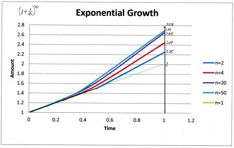
The graph on the right plots the savings amount for the different “deals”, with different n-s. It is a plot of A versus the interest payment time. Note that as n increases, the curves lift up more and more near the year end. They are more than double the simple interest case even though the interest rate is still 100% per year. Compound interest definitely makes more money for you than simple interest (n = 1).
We have been considering the saving duration to be one year, but the argument holds for any saving period. The interest rate would be the “total” rate over the whole duration.
What if the bank gives an interest rate of r, instead of 1? The formula will become
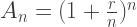
r is the total rate of interest over the whole duration of the saving.
n is the total number of payment times over the whole duration.
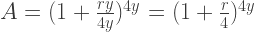
Example – Say, the bank offers quarterly “compounding” frequency, i.e. 4 times a year.
We save over y years. To get a formula for the amount over y years, we determine:
Number of interest payment in y years = n = 4y
Total interest rate over y years = ry
We get
For the general case of compounding n times a year,

This is the familiar formula for compound interest.
You can verify that the more often they give interest (increase n), the more your saving will increase. 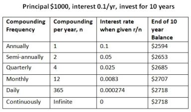
The table illustrates an example of compound interest on principle of $1000 over 10 years. The interest rate is 0.1 per year.
For the above equation for A, this is P = 1000, y = 10, total interest rate = r = 0.1•y = 1.0, #interest payment = n•y. We consider the cases where the bank compounds more and more often, from annually down to daily. Note that when the bank gives out interest twice a year, the rate each time would be half the annual rate. That’s why the factor r/n in the formula. This reduced interest rate is made up by receiving the interest more often. So we see that the balance at the end of 10 years grow each time.
But that is not all 🙂
Mathematicians are always interested in “pushing limits”, they wonder “what happens if n goes to infinity, i.e., the bank gives interest “continuously”, never pausing. As we saw above, the total interest increases with bigger n, so n going to infinity would be mean that the bank gives you the maximum interest (with the same total interest rate). Of course, that is never going to happen, but mathematicians like to post questions and solve puzzles. So they examined the above equation to push its limit (literally n -> infinity):
They pushed the equation:
They were able to calculate the limit and fill in the last row of the table.
To their delight, mathematicians found that the expression 
$latex e =
so the above equation for A become simply:
Note that the definition of e does not include any information on the bank interest problem. In fact, it is independent on the application problem at all. This value of e can be used in all the applications with the above definition expression.
Wow, what a treat 🙂
To honor Leonard Euler (1720), e is called the Euler’s Number.
This number has many wonderful properties, it became most useful in math and sciences. We described some of them in the section New Numbers.
