Many Numbers

Many Numbers together

Numbers are interesting, but examining a group of numbers together reveals more interesting ideas. We look how the individuals relate to each other and at the group’s property as a whole. The following are examples of some number groupings.

Sequence and Series

Let us first consider a list of numbers, one after another:

A = 0, 3, 6, 9, 12, 15

This, A, is called a Sequence. The order of the numbers is important, so it is formally called “ordered sequence”, though often the word “ordered” is assumed. A Series is the sum of a sequence, for example, if we add the above sequence, we get Series SA:

SA = 0 + 3 + 6 + 9 + 12 + 15

Examining the sequence A, we see that the difference d between two neighboring elements is always the same number 3. This constant “first difference” classifies this sequence as an Arithmetic sequence, and the series SA as an Arithmetic series.

A different example is the following sequence and series:

G = 2, 4, 8, 16, 32, 64

SG = 2 + 4 + 8 + 16 + 32 + 64

The elements in sequence G do not have a constant first difference. In fact each element is a multiplying factor r from the previous element, i.e., 4 is double 2, 8 is double 4 etc. This factor is the same down the sequence elements. This sequence is called Geometric, and the series is a Geometric series.

The elements of the geometric sequence G can be written in the exponential form $2^n$ , where n = 0, 1, 2, .. labels the order count of the sequence.

Examples of geometry sequence are common, here are a few:

Moore’s Law: the number of transistors on a chip doubles every two years while the costs are halved.

Facebook friends count: Assume you have 100 Facebook friends, and each of them have 100 friends, that would amount to 10000 “Friend of Friends”. For Facebook’s 3rd degree of separation, that would be 1,000,000 friends. The counts grow fast (exponentially!) Similar results apply to tweeting and retweeting counts.

Compound interest: Assume you save money in a bank with an initial principal of $100 and you get interest (bank pays you) 5% per year. At the end of the year, you will have $100•(1.05) = $105. An interest of $5 has been added to the principal of $100. What happens next depends on whether the bank gives you simple interest or compound interest.

If the interest is simple, $5 will be added every year to your account, it’s that simple. If the interest is compound, your interest gain will be calculated based on what is total in your account at that time. At the end of the year, you have $105, the new interest will be 5% of that for one year. Thus at the end of the second year, the interest gain would be $105•(0.05) = $5.25, and you will have $105•(1.05) =$110.25 in your account. This can be written as $100•(1.05)•(1.05). As years pass by, your account will be the sequence:

100, 100•(1.05), 100•(1.05)•(1.05), 100•(1.05)•(1.05)•(1.05), …

which calculates to: 100, 105, 110.25, 115.76, 121.55, …

You see the amount in your account increases by a factor 1.05 every year. It grows faster than a constant interest simple interest. In short, the equation for saving after y years (assuming you do not take any money out) is:

$A = 100 (1 + .05) ^y$

This equation gives the sequence displayed above.

For more information on compound interest and exponential growth, please go to the page Exponents and Logarithms.

Simple Statistics

Statistics is a mathematical subject which deals with collections of data as a whole. It is not interested in the individual data, but the whole population.

Consider a sequence of numbers $x_1, x_2, x_3, .. x_n$ , here are some simple statistical results:

Sum $S = \sum_{i=1}^n x_i = x_1 + x_2 + x_3 + .. + x_n$ ,

Mean $\mu = \frac{1}{n} S$ ; Variance $\sigma^2 = \frac{1}{n} \sum_{i=1}^n (x_i - \mu)^2$

Some statistical results for series considered above:

For arithmetic series: Sum SA = $n(a_1 + a_n)/2 = n(2a_1 + (n-1)d)/2$

For geometric series: Sum SG = $a_1 (r^n - 1) / (r - 1)$

We will explore statistics in more detail in another page, here.

Fitting Data

The figure on the right displays data scattered over the “sca Linear_fit_1 tter plot”. The scientist, who collected the data, wished to make a model to explain the data collected. Her first attempt was to find a straight line to “best fit” the data. She did it “by eye”.

The displayed red line appears to go through the “center” of the data, having approximately equal distance from the data on either side. The problem is how to accurately find the equation for this “Best Fit straight line”.

Assume the line has the equation is y = mx + b, where m is the slope, and b is the y-intercept. We want to determine m and b. Let $(p_x, p_y)$ be the data points.

One criterion for “Best Fit” is to minimize the separation between the line and the data points. We can sum the vertical differences (named residuals or “errors”), but that would be zero, because there are equal separations above and below the line. So we sum the squares of the errors and try to find a line which makes that sum of error-squares as small as possible.

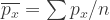
But before we do that, we want to simplify the analysis. We shift the origin of the plot to the centroid of the data, i.e. the mean values of the data $p_x$ and $p_y$ . The centroid location is at $(\overline{p_x}, \overline{p_y})$ . If n is the number of data points, $\overline{p_x} = \sum p_x /n$ , $\overline{p_y} = \sum p_y) / n$ .

After the origin shift, the best fit line will go through the origin and has the simple equation y = mx. We compare where the formula places the x-value point $p_x$ to the actual $p_y$ of the data. The error at that data point is $(p_y - mp_x)$ .

The sum of squares of error is then:

$S_e = \sum(p_y - mp_x)^2 = \sum p_y^2 - 2 m \sum p_y \sum p_x + m^2 \sum p_x^2$

The expression on the right side is a quadratic in m. It can be rewritten as

$S_e = C_0 + C_1 m + C_2 m^2$ ,

where $C_0 = \sum p_y^2$ ; $C_1 = - 2 \sum p_y \sum p_x$ ; $C_2 = \sum p_x^2$

Now, we learned from the page on Parabola that a parabola with a formula 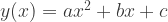$y(x) = ax^2 + bx + c$ has its minimum y value (apex) at the independent variable location $\frac{-b}{2a}$ . (A better explanation is in the page “Differentiation” of the Calculus section). Applying this to the above, we got the minimum value of $S_e$ is reached at value of m as:

$m = \frac{-C_1}{2C_2} = \frac{\sum p_y \sum p_x}{ \sum p_x^2}$

Now, the final step (whew) is to shift the origin back from the data centroid $(\sum p_x /n, \sum p_y /n)$ .

So the line with function y = mx would be moved up by $\sum p_y /n$ and moved right by $\sum p_x /n$ . Remembering how the formula is changed when its graph is moved, the restored best fit line formula is:

y = $\frac{\sum p_y \sum p_x}{ \sum p_x^2} ( x - \sum p_x /n) + \sum p_y /n$ .

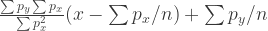
Note: As we will learn in the section on Calculus / Differentiation, there is a simpler way to calculate the minimum value.

Infinitely Many

One way mathematicians like to “push the limit” of their imagination is to consider infinity, symbolized by ∞.

We encountered one example of this when we discussed Compound Interest. There we considered what happens when the bank gives you interest compounded “continuously”. Then the number of interest payment is allowed to go to infinity, and the account is given by $A = P \cdot \lim_{n\to \infty} (1 + \frac{r}{n}) ^{ny}$ . The saving thus grows exponentially with the Euler number e as base: $A = P \cdot e ^{ry}$ .

Another well known example is inspired by Zeno’s (430 BC) paradox, Zeno_Dichotomy_Paradox as follows:

Before you can walk home, you must get to the half-way point. From there, you must get to its half-way point to home (1/4 way more), etc. See picture. It will take you “forever” to get home!

Fortunately, mathematicians came to rescue. This is an example of an infinite series: a series with infinite number of terms. In this case, if we let the distance to home be 1, the “steps” to walk home would be the sum:

S = $\frac{1}{2} + \frac{1}{4} + \frac{1}{8} + \frac{1}{16} + ...$

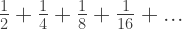
where … means the terms are to be continued, indefinitely.

To calculate this, we use a trick that relies on the infinite number of terms. First we multiply S by 2, getting:

2S = $\frac{2}{2} + \frac{2}{4} + \frac{2}{8} + ...$ = 1 + $\frac{1}{2} + \frac{1}{4} + ...$

The trick is to realize that the last part of this equation is 1 + S.

So 2S = 1 + S. Thus S = 1.

This can be written as: Sum = $\sum_{n=1}^\infty \frac{1}{2^n}$ = 1.

Hurray, you can finally get home 🙂

There are many examples of infinite series with stunning and unexpected results. The following are some of them. They are included to wet your appetite. You may do some research to find out more details:

$e = \frac{1}{0!} + \frac{1}{1!} + \frac{1}{2!} + \frac{1}{3!} + \cdot \cdot \cdot$ .

$\frac{\pi}{4} = 1 - \frac{1}{3} + \frac{1}{5} - \frac{1}{7} + \frac{1}{9} - \cdot \cdot \cdot$ .

$\frac{\pi}{6} = \frac{1}{1^2} + \frac{1}{2^2} + \frac{1}{3^2} + \frac{1}{4^2} + \cdot \cdot \cdot$ .

To learn more about infinite series and whether they converge, see here.

Infinitely Small

Mathematicians are also interested in pushing the limit to the other extreme, to zero. We saw this in the section of Rate of Change, when we discussed “instantaneous slopes”. There the instantaneous slope is found by the formula:

$\frac {dy}{dx} = \lim_{\Delta x\to 0} \frac{\Delta y}{\Delta x}$

where Δx is shrunk to 0 in the limit.

More will be discussed in the page Calculus.